The goal of our project is to simulate gradient light emission from heated metal objects. We will model how heat and the resulting glow varies over a surface, with consideration of material attributes.
Problem Description
From the experiences that we've had applying glow attributes to models in 3D programs such as Autodesk Maya (used with Pixar RenderMan), we've found that the results fail to take into consideration material properties and variations in heat across a surface. Thus, they cannot be used to accurately represent objects that emit energy and glow.
Through this project, we aim to create functionality for a realistic representation of heated objects with diverse metal material properties. By doing so, we will demonstrate the different ways light emission can be simulated when considering the energy absorbance and reflectance properties of different materials.
Using guidance from a few papers we are reading on, we plan to work through this problem by considering blackbody radiation models based on Kirchkoff's law.
Goals and Deliverables
Through our analysis, we hope to gain understanding of how heat emittance varies between different materials and temperatures.
Quality and Performance
To measure the quality of our system, we will compare our renders to photographs of actually heated objects of different materials. To measure the performance of our system, we will compare the time it takes for a glowing object to light a scene against the time it takes for a typical light source to light a scene.
Plan to Deliver
We plan to deliver several images comparing the heated glows of at least three different metal materials. This can be done by considering the different energy absorbance/reflectance values of various materials that contribute to the resulting heat representation. We also plan on simulating the gradient glow of an object with non-uniform heat distribution (parts of the object are hotter or cooler than other parts). This can be done by interpolating glow gain values over a heat map.
Hope to Deliver
If we have extra time, we would like to consider how we might turn this into a plugin for a current existing 3D modeling or rendering software, such as Autodesk Maya.
Additionally, we hope to provide animated simulations of time-varying heat maps as the heat and corresponding glow of an object changes over time.
Interactivity
Our goal is for the program to take JSON files defining material attributes, PNG files acting as UV heat texture maps, and COLLADA (.dae) files defining 3D objects, and output a rendered PNG image.
Schedule
| Date | Tasks |
| 4/11 | Frameworks, shader files, and object models set up. Finalize technical descriptions of the components of the paper(s) we intend to replicate and expand upon. |
| 4/15 | Create glow functionality based on material properties and temperature. Implement toggling of shader components: diffuse emission, reflectance, and absorption according to Kirchoff's Law. |
| 4/22 | Implement temperature textures, possibly time-varying (animated). Complete the file input interface. |
| 4/28 | Status report webpage, slides, and video. Renderings demonstrating our work. |
| 5/6 | Presentation slides. Structure and basic content of the final webpage. All coding finalized. |
| 5/12 | Finalized video and webpage. |
Resources
- Our own computers
- Hive machines
- Project 3 codebase and renderer
- A Physically Plausible Model for Light Emission from Glowing Solid Objects
- Visual Simulation of Heat Shimmering and Mirage
- Autodesk Maya and/or Blender for creation of example COLLADA files
Diffuse Blackbody Emission
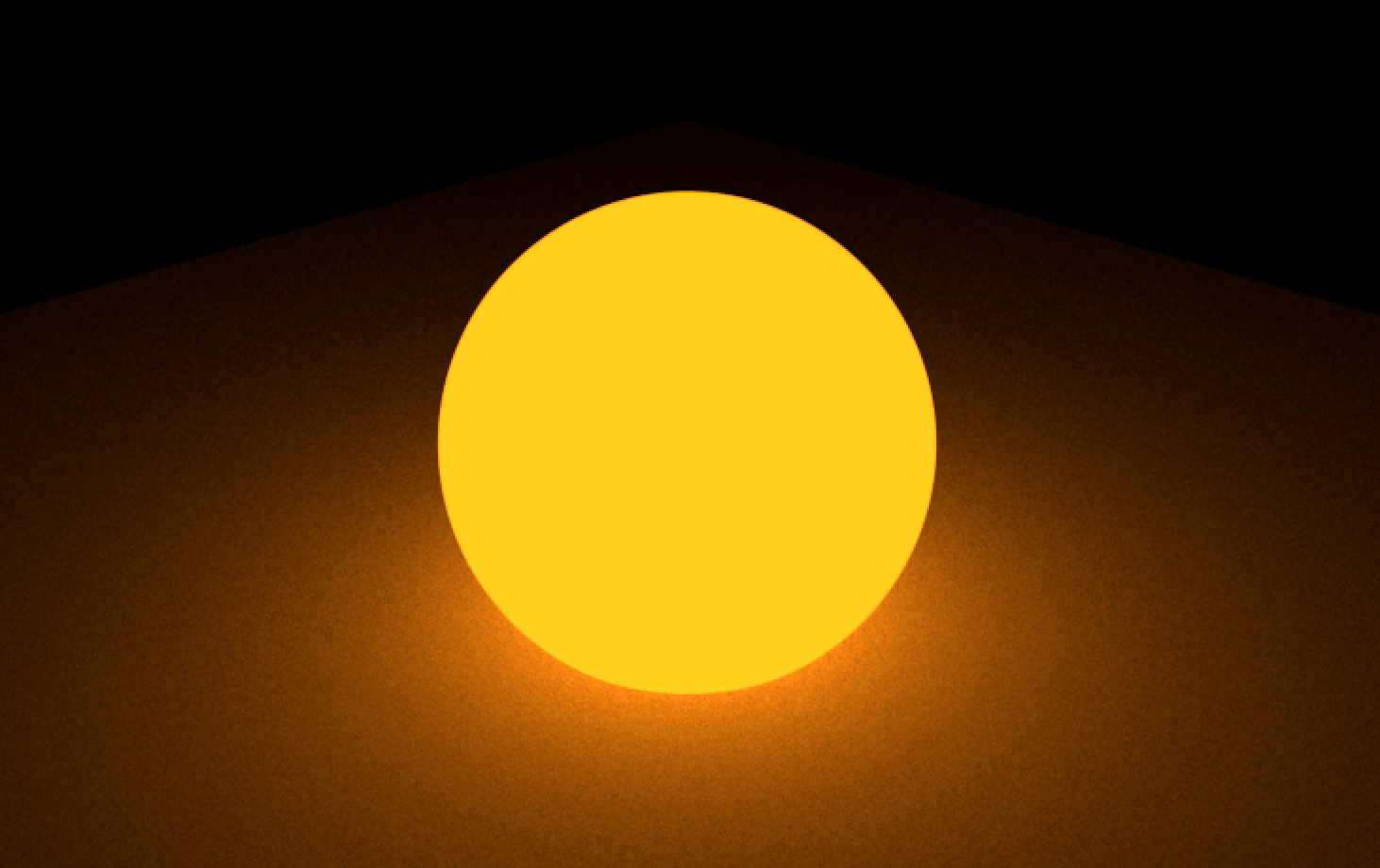
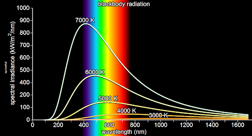
We start by implementing the glow of perfectly diffuse emissive objects for some input temperature. In this case, our object is an ideal blackbody that absorbs and re-emits all energy falling upon it. We find the spectral radiance of our blackbody through Planck's law of black-body radiation.

Using this equation, we calculate a distribution of 81 discrete wavelengths ranging from 380 - 780 nm, roughly the human visual spectrum. Then, in order to compute a final color compatible with the computer display, we first convert the high dimensional spectrum to the three dimensional CIE 1931 XYZ color space, then apply a transformation matrix and gamma function to convert to sRGB.
Reflectance
In order to realistically render gradual changes in glow color as temperature varies, we combine our estimate of blackbody radiation with the microfacet-model reflectance of the metal. The final sampled color is a combination of reflected and emitted light, weighted by the absorbance factor of the material (1 - reflectance). Kirchoff's Law of Thermal Radiation ensures that the energy of the system is conserved, resulting in more realistic renders.
Kirchoff's Law: At thermal equilibrium, the emissivity and the absorptivity of a surface at a given temperature and wavelength are equal
Test Renders
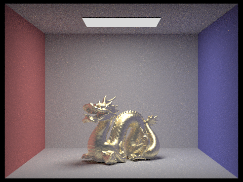
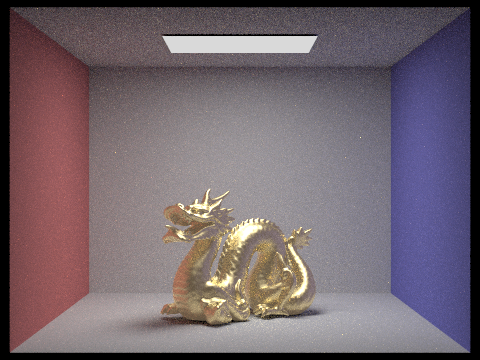
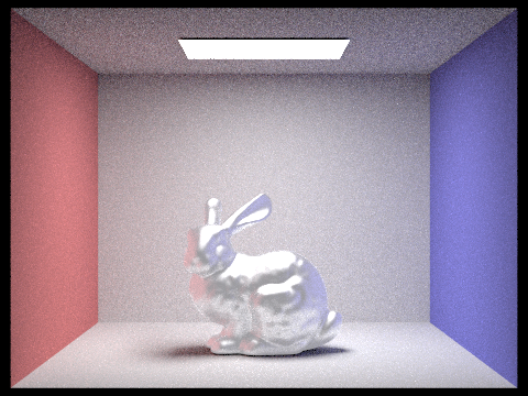
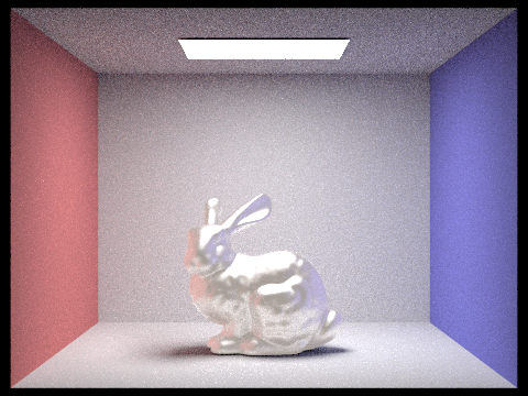
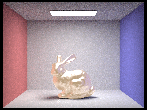
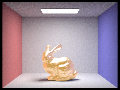
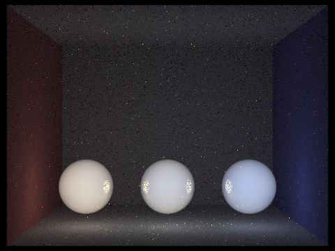
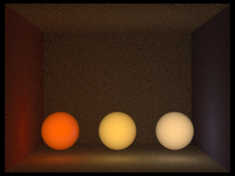
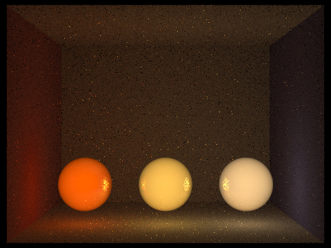
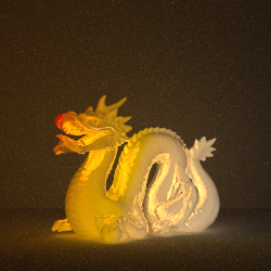
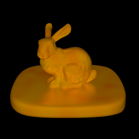
We used reflectance data from this website to estimate an average reflectance factor for each material (3D Shelf, 614 nm, 0° incidence). Our renders demonstrate temperature-responsive glow, direct illumination only (for now).
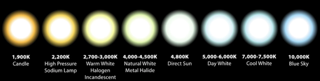
Our input temperature varies along the Kelvin temperature scale:
Gold dragon, reflectance factor = 0.9


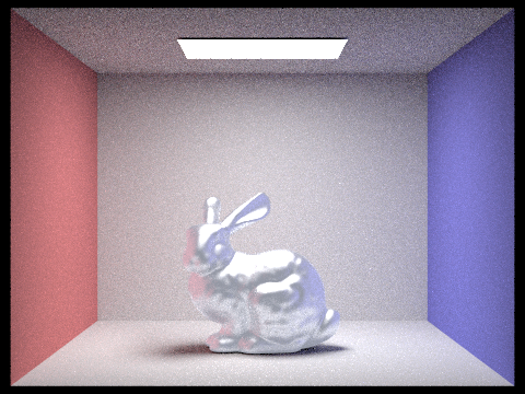
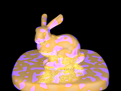
Lead bunny, reflectance factor = 0.6
Fresnel Terms
As we plan to take into consideration the effect of polarized light, we've split up the Fresnel reflectance coefficient calculations into s polarization and p polarization.


Process
So far we've modified the aforementioned quantities in a new BSDF class, called GlowingBSDF. We've also modified the estimation of global illumination by replacing the zero-bounce-radiance with the blackbody radiation weighted by the absorbance -- this allows us to simulate the glowing of the material.
Reflection
We're slightly behind the progress goals set in the proposal, but we've already produced some nice renders with the features implemented so far. We still have plenty of time to implement the most important features that remain.
Next Steps
Right now, our renders only demonstrate the direct illumination of the glow effect. We will work on tracing multi-bounce paths to achieve global illumination. We also aim to render objects with non-uniform heat distributions by interpolating glow gain values over a heat map.
Final Presentations
Milestone Presentations
Abstract
The Problem
From the experiences that we've had applying glow attributes to models in 3D programs such as Autodesk Maya (used with Pixar RenderMan), we've found that the results fail to take into consideration material properties and variations in heat across a surface. Thus, they cannot be used to accurately represent objects that emit heat/energy and glow.
The Solution
For this project, we created functionality for a realistic representation of heated objects with diverse metal material properties. By doing so, we are able to demonstrate the different ways light emission can be simulated when considering the energy absorbance and reflectance properties of different materials. We also modeled how heat and the resulting glow could vary over a surface, by implementing volumetric temperature maps.
Technical Approach
This project was built as an extension of the Project 3 Pathtracer codebase.
Diffuse Blackbody Emission
We start by implementing the glow of perfectly diffuse emissive objects for some input temperature. In this case, our object is an ideal blackbody that absorbs and re-emits all energy falling upon it. We compute the spectral radiance of our blackbody through Planck's law of black-body radiation.
Using this equation, we calculate a distribution of 81 discrete wavelengths ranging from 380 - 780 nm, roughly the human visual spectrum.
Reflectance
In order to control the glow attributes and inputs for different meshes, we create a GlowingBSDF class that expands on the microfacet model seen in Project 3. Here, we combine our estimate of blackbody radiation with the reflectance input of the metal, allowing us to realistically render changes in glow color as the temperature and metal material of our objects vary. The final sampled color is a combination of reflected and emitted light, weighted by the absorbance factor of the material (1 - reflectance). Kirchoff's Law of Thermal Radiation ensures that the energy of the system is conserved, resulting in more realistic renders.
Kirchoff's Law: At thermal equilibrium, the emissivity and the absorptivity of a surface at a given temperature and wavelength are equal
Color Reproduction
To compute a final color compatible with the computer display, we first convert the high dimensional spectrum to the three dimensional CIE 1931 XYZ color space, then apply a transformation matrix and gamma function to convert to sRGB.
Polarization of Light
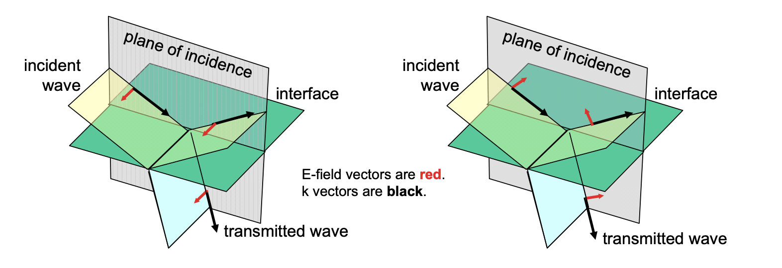
Experimenting with the polarization of light and how that might enhance our glowing effect, we tested out both dielectric-dielectric and dielectric-conductor Fresnel terms split between both s and p polarization. In differentiating S (perpendicular) polarization and P (parallel) polarization, the electric field is either perpendicular or parallel to the plane of incidence -- the plane that contains the incident and reflected wave vectors.
Ray Tracing Glowing Objects
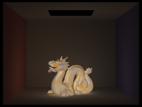
To achieve both direct and global illumination, we altered the get_emission function of our GlowingBSDF class to return a radiance Spectrum based on the direction of the incoming light ray and the temperature at the point of ray intersection. This allows us to simulate the glowing effect while visually preserving the object’s dimensionality.
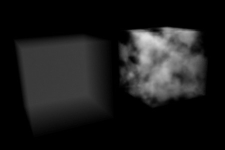
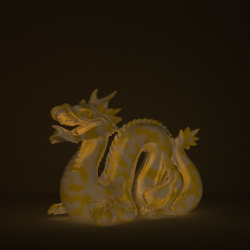
Volumetric Temperature Maps
Additionally, we modified our COLLADA parser, allowing it to read a temperature distribution tag that could process either a constant temperature, a linear gradient map, or a Perlin noise map. The code used to compute the Perlin noise function itself was found here, based on the original paper by Ken Perlin.
For a constant temperature, we apply a uniform temperature distribution throughout the entire mesh, based on a scalar temperature input.
For our linear gradient map, we obtain smoothly varying temperature values across the surface of our mesh through linear interpolation of two start and end temperature inputs at corresponding 3D vector positions.
For our Perlin noise map, we apply the Perlin noise function to obtain a pseudo-random temperature distribution ranging between two input temperatures. Another input controls the noise fineness -- how quickly the temperatures fluxuate across 3D space.
Spectrum Caching
In order to improve program efficiency, we implemented a dynamic caching system that stored a map from integer-rounded temperatures to RGB Spectrums, reducing the amount of computation needed for repeated temperature samples.
No loss in image quality was detectible due to rounded temperature samples, as the bucket size is very small in comparison to the wide range of possible temperatures. Further research could determine the effectiveness of larger and/or adaptive bucket sizes, as greater temperature gaps are required to produce a visual difference in emission as overall temperature increases.
Using our caching system, slight but consistent improvements in render speed were observed with a variety of models, materials, sampling rates, and temperature distributions.
| Temperature distribution | Render run time... | Sampling rate (samples/pixel) | ||
|---|---|---|---|---|
| 1 | 8 | 64 | ||
| Constant | w/o caching (s) | 0.593 | 4.737 | 24.760 |
| w/ caching (s) | 0.558 | 4.091 | 23.249 | |
| Improvement | 6% | 14% | 6% | |
| Variable (noise) | w/o caching (s) | 0.693 | 4.609 | 24.625 |
| w/ caching (s) | 0.534 | 4.243 | 23.307 | |
| Improvement | 23% | 8% | 5% | |
Problems Encountered
Out-of-gamut colors for low temperatures (<2000K)
We were not initially able to reproduce the reddish emission color of objects heated to temperatures less than about 2000K, instead producing a range of strange pink hues. Converting from CIE XYZ to sRGB, we found that the resulting Spectrum sometimes contained a red value greater than 1, and a blue value less than 0. By clamping these values to the range 0 through 1, as required by the Spectrum class, this problem was fixed.
Ray Tracer Modifications
Our first attempt at ray tracing glowing objects didn’t work without external lighting, as the path tracer was importance sampling only light objects for one-bounce illumination. Also, zero-bounce illumination was only capable of returning a constant radiance from a BSDF, with no dependence on ray direction or intersection position. At this time, we only had access to Project 3-2 code, so we couldn’t directly change these aspects of the path tracer code.
In our second attempt, we ported in Project 3-1 code and changed the zero-bounce radiance code and our GlowingBSDF get_emission function to return a direction and position dependent emission. This blackbody emission was multiplied by an average absorbance factor, as described in the paper. We also altered our code to use cosine hemisphere sampling so the glowing objects could produce global illumination.
Lessons Learned
Alongside overcoming the problems we encountered in the previous section, we learned a lot about the physics behind glowing objects, from blackbody radiation and Kirchoff’s Law to polarization. Applying the concepts we learned in the color reproduction lectures really helped us understand the computational representations of color.
Going through the project, we also strengthened our understanding of how the Project 3 Codebase worked, from following an XML file through the Collada Parser, to ray-tracing and incorporating the BSDF functions.
This process also familiarized us with working in a team across Github and XCode -- from fixing small linker issues to modifying the Cmake List and rebuilding when we create new files. It was interesting to go through iterations on our project -- dropping by office hours when we got really stuck and going back to edit the code to work with advice we’d received.
Results
Varying Temperatures

Polarization of Light

Optical Material Properties
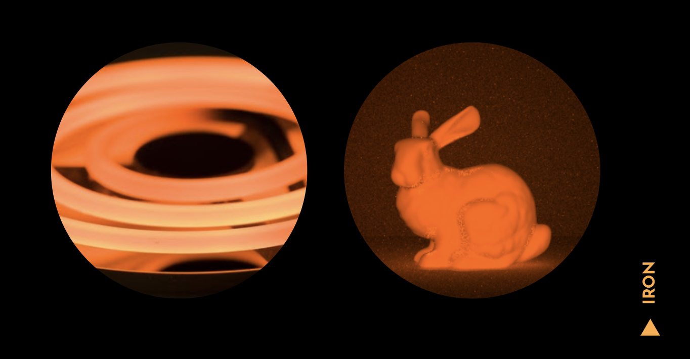
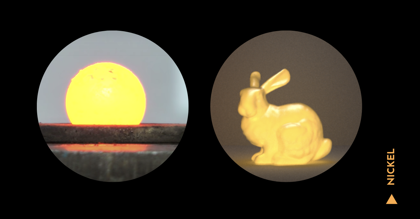
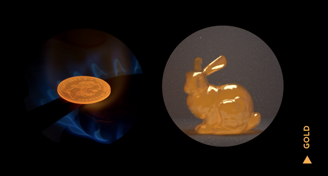
We used reflectance data from this website to obtain the reflectance and Spectrum values of specific metal materials in an attempt to produce realistic renders. From here, we compared our renders to photographs of real heated metals.
Volumetric Temperature Maps
Linear gradient map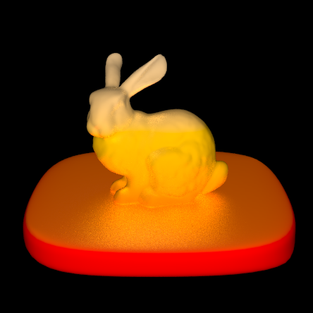
References
- A Physically Plausible Model for Light Emission from Glowing Solid Objects (A. Wilkie and A. Weidlich)
- Improving Noise (K. Perlin)
- Perlin noise in C++11 (P. Silisteanu)
- How to convert between sRGB and CIEXYZ
- CIE Colour Matching Functions
- Fresnel equations
- Refractive Index Database
Contributions
Ethan Buttimer
- Set up GlowingBSDF class and added support to parser
- Created SpectralDistribution class and implemented color conversion from spectral distribution to CIE XYZ and sRGB Spectrum
- Created the volumetric temperature distribution framework and added support in parser for three types of distributions
- Integrated Perlin Noise into the renderer through the temperature sampling function of the NoiseTempMap class
- Implemented and tested Spectrum cache
Jen Hoang
- Implemented Planck's equation for computation of the spectral distribution for blackbody diffuse objects
- Computed interpolating temperature values in 3D space for linear gradient distribution
- Made XML file modifications for material data and linear gradient renders
- Designed and made webpage
Susan Lin
- Worked on GlowingBSDF functions, especially with the Fresnel term in relation to polarization
- Modified XML files for material data and varying temperature renders
- Compiled, recorded, and edited videos